
Understanding Word2Vec With PySpark
Published:
Understanding Word2Vec with PySpark
Goal
I need to use word embeddings to study the evolution of hate speech across social media. I chose to explore Word2Vec in hopes of learning more about it and to begin to probe the field of Natural Language Processing.
Today we are going to look at how Word2Vec incorporates word embeddings to create a numeric vectors to represent meaning of words. This is an important part of natural language processing (NLP). The goal of NLP is to extract meaning from human language, often this is provided in the form of text. And this meaning can be found in many components of language.
Some components of language
- Pragmatics
- Semantics
- Syntax
- Morphology
- Phonology
Dataset
I am using a Gab.ai dataset of posts submitted to the social platform. Gab.ai prides itself on the values of “free speech” and a lack of censorship. As a result it has become known for attracting trolls, bots, and the socially maligned. Comments and posts made to this site are notorious for being extreme and hate laden. I have collected over 28 million posts and will use a 1 million post sample to train a skip-grams variant of the word2vec word embedding model. The goal is to identify the proximity of two related words in a vector space.
Distributional Semantic Models
Word embeddings are word representation algorithms used in an NLP. Word embeddings are a subclass of distributional semantic models because they rely on the distributional hypothesis. The distributional hypothesis, created by Zellig Harris in his 1956 paper “Distributional structure” , is assumption that words in the same context tend to proport similar meanings and occur near each other. And thus synonyms have similar representations in a collection of texts. Word embeddings are represented as vector values created as a result of a neural network.
Example Posts
data.body
"Probably because I see the faint hint of 'horns' holding that halo up... "
https://youtu.be/YMQRFT4bZuc
http://www.epochtimes.de/politik/europa/zahl-der-toten-nach-londoner-hochhausbrand-auf-79-gestiegen-2-a2146594.html
https://t.co/LTMBeXvHrC
"Ps 37:14 Die Gottlosen ziehen das Schwert aus und spannen ihren Bogen, daß sie fällen den Elenden und Armen und schlachten die Frommen.\nPs 37:15 Aber ihr Schwert wird in ihr Herz gehen, und ihr Bogen wird zerbrechen.\n\n"
At least 25 killed in airstrike on market in Yemen – reports\nhttps://www.rt.com/news/392838-saudi-yemen-market-airstrike/ #saudiarabia #yemen
Example after cleaning
['data', 'body']

['', 'probably', 'because', 'i', 'see', 'the', 'faint', 'hint', 'of', "'horns'", 'holding', 'that', 'halo', 'up', '', '', '', '', '']
['https', '//youtu', 'be/ymqrft4bzuc']
['http', '//www', 'epochtimes', 'de/politik/europa/zahl', 'der', 'toten', 'nach', 'londoner', 'hochhausbrand', 'auf', '79', 'gestiegen', '2', 'a2146594', 'html']
['https', '//t', 'co/ltmbexvhrc']
['', 'ps', '37', '14', 'die', 'gottlosen', 'ziehen', 'das', 'schwert', 'aus', 'und', 'spannen', 'ihren', 'bogen', '', 'daß', 'sie', 'fällen', 'den', 'elenden', 'und', 'armen', 'und', 'schlachten', 'die', 'frommen', '\\nps', '37', '15', 'aber', 'ihr', 'schwert', 'wird', 'in', 'ihr', 'herz', 'gehen', '', 'und', 'ihr', 'bogen', 'wird', 'zerbrechen', '\\n\\n', '']
['at', 'least', '25', 'killed', 'in', 'airstrike', 'on', 'market', 'in', 'yemen', '–', 'reports\\nhttps', '//www', 'rt', 'com/news/392838', 'saudi', 'yemen', 'market', 'airstrike/', '#saudiarabia', '#yemen']
Now we have to take this tokenized text and use this as our input text
Building a Vector
To use the distributional hypothesis to build a vector, we have to choose what words being near each other means to us. This value of “nearness” is known as a window. In the image below, taken from Chris McCormick’s tutorial, the target word is highlighted in blue, and the window shown around it as being two words away from the target. This means the window size is equal to 2. 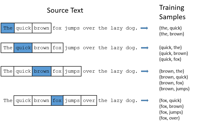
Word pairs are created between the target word and all other words in the window which can extend forwards or backwards. The target is then moved to the next word and the process repeats. Some embedding models treat words to the left of the target word differently than words to the right. But for now we will treat them both equally.
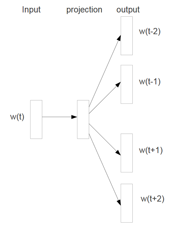
Figure 2: A diagram of the skip-gram model for starting with the target word and trying to predict the context words which are the words in the window: This image was taken from Tomas Mikolov et al’s original paper: Distributed Representations of Words and Phrases
These word pairs become the training samples for the model. We will be using the key of this pair to create what is known as a one-hot vector. Currently they are in the form of (target word, context-word-in-window) and this will be used as the input for a simple 1 hidden layer neural network. In Figure 2 above, the target word is W(t). The projection of the input onto a hidden layer of which has a pre-determined number of neurons that was specified as a hyper parameter. A hyper parameter is the number of hidden layer neurons has a large effect on the accacury and speed of the model’s runtime and 300 is widely used in practice since it was used by word2vec’s creators. This simple neural network is known as a Restricted Boltzmann Machine (RBM).
Restricted Boltzmann Machines (RBMs)
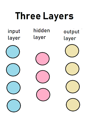
In the image above, there are three columns that are known in discriptions of neural networks as layers. These diagrams show cause and effect between the layers of a neural network and are read from left-to-right. Each circle represents a neuron and is called a node. A node is where a calculation is preformed to determine if it will send a 0 or a 1 to a node in the next layer, which is to the right. This communication is known as firing and only happens in one direction, left-to-right.
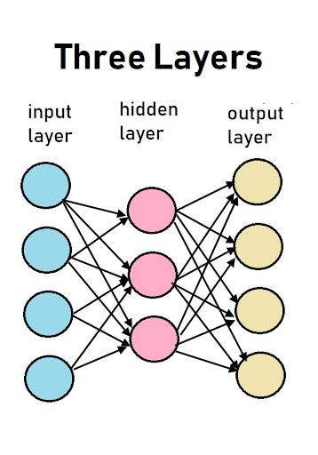
In our restricted boltzman machine, nodes are not linked to, or communicate with, other nodes within the same layer. This restriction gives the RBM its name. And every node in the input layer is linked to each node in the hidden layer. The nodes/neurons in the input layer are considered to be different neurons in the hidden layer, hence why they are in different layers.
I stress this point because this is known as a bipartite graph. But not just any bipartide graph, a complete bipartite graph because these two layers are fully linked. Note, that some texts call this a symmetrical bipartite graph. Also it is important to notice in the graphic above how the hidden layer has fewer nodes than the input or output layers. This is an important quality of RBMs as a feature known as dimensionality reduction.
When a RBM is inalitized, four things are determined in advance and thus are hard-coded into the construction of the neural network. This things are known as hyper parameters.
- Number of nodes in the input layer
- Number of nodes in the hidden layer
- Number of nodes in the output layer
- The weights of the nodes in the hidden layer
With RBMs a special step happens when the hidden layer is created. Each node is randomlly assigned a weight. A wight is the power that node has on the nodes it is linked to in the next layer. This process of randomlly assigning weights is known as Stochastic Gradient Descent. It is called this because stocastic means “random” and these weights provide influence on the node in the next layer they are linked to.
The random assignment of the weights for word2vec is only done on the first round. The entire neural network is trained multiple times. Each one of these training rounds is called an Epoch. The weight matrix from the previous round is used as the initial weight table for the next round.
These weights are important to Word2Vec and like normal RBMs, Word2Vec randomly assigns weights. Word2Vec adjusts these weights over time while the neural network is fed our one-hot vector we created from our word pairs. This is known as training the neural network. Word2vec is similar to an autoencoder, as it encodes each word into a vector. But rather than training against the input words through reconstruction, as a restricted Boltzmann machine does, word2vec trains words against other words that are found in the context window of the input corpus.
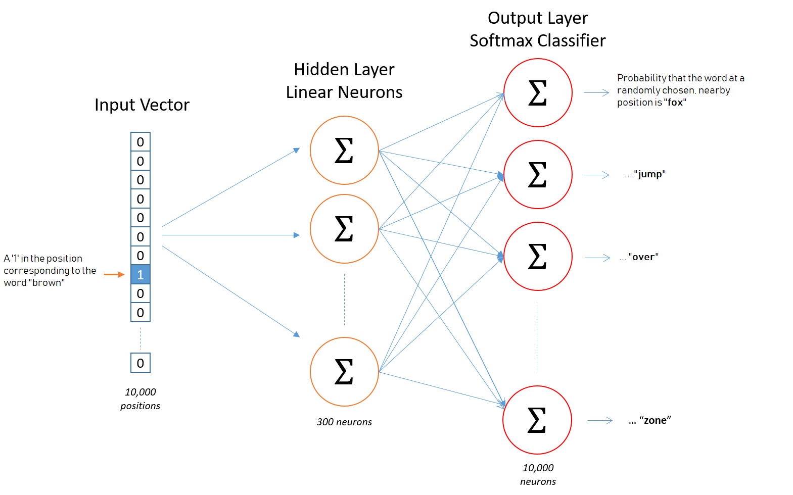
Figure 4: This image was adapted from Chris McCormick’s Word2Vec Tutorial - The Skip-Gram Model tutorial
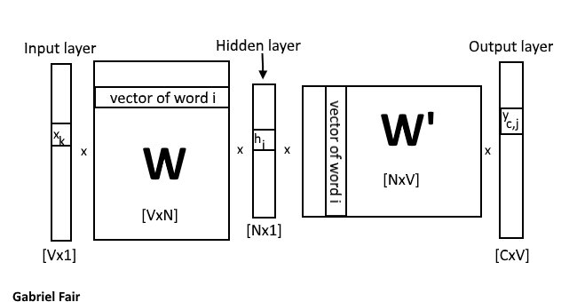
Figure 5: A diagram of how word2vec uses linear matrixes to train its neural network
Understanding Figure 5, the linear algebra of Word2Vec
Above I explained how the network is trained many times. The same input is fed into the network each time but the weight matrixes from the previous round is used as the inital weight matrix for the next round. In Figure 5, this is matrix W.
So for our first round we will start with
h=xTW
Since x is a one-hot encoded vector, h is simply doing a lookup of the kth row of the weight matrix W. Each row becomes a hidden layer for each word via the lookup trick provided by the one-hot encoding.
yc,j= W′Th
so essentally the output element is just the transpose of the weight matrix between the input and hidden layer and the hidden layer and the output layer. so
yc,j = W′TWTx
But there is one step missing from this equation above. The final output vector needs to be softmaxed. This takes the output layer (Y) and compresses the values into the range between 0 and 1. This allows for Y to act as a probability distribution for the input words (X). The equation for softmax is below:
We are using softmax since it continuous output provides a good use case for multiclass classification
I have trained using the method explained above. I used only 100 nodes in my hidden layer. The model would be more accurate if it was trained on a larger hiden layer. Often the size of this layer is 300 nodes.
Explaining skip-gram
Create list of predicted words for the target word ‘trump’
print(model_vectors['trump'])
[0.012244515, 0.05669574, 0.4243817, -0.13005282, 0.14591245, 0.15754509, 0.12144023, -0.043377433, -0.036471862, -0.17795071, -0.15042417, 0.4285602, -0.16748007, -0.09618644, 0.07635299, 0.021112783, -0.1097202, 0.16649377, 0.31761286, 0.2781521, 0.26321766, -0.35739362, -0.17595355, -0.28173986, 0.2220869, 0.421465, 0.12334027, 0.17061687, -0.16097873, 0.1101991, 0.39143816, -0.10224187, 0.19060156, 0.06379647, -0.055479944, 0.30508712, -0.33523571, -0.3099334, 0.16205992, 0.23172502, 0.12932838, -0.25712037, -0.24778262, -0.41348562, 0.10876833, -0.095286794, -0.12277438, 0.08167293, 0.2416396, -0.29519707, 0.07202256, -0.03740526, -0.08972215, -0.03250894, -0.21824007, 0.04827257, -0.009086915, 0.18352096, -0.10135367, -0.47981852, -0.06576853, 0.021472175, 0.023349164, 0.05336668, -0.37836334, 0.08596835, -0.08231194, -0.09812828, 0.0058923, -0.06080334, 0.15352124, 0.2911331, 0.15038647, 0.15921666, 0.13570379, 0.09163106, 0.0093092015, 0.0024938602, 0.16191821, -0.116921216, 0.37449756, -0.37325835, 0.17355393, 0.22919315, -0.22791475, -0.12990569, 0.15548478, -0.16302991, 0.09529176, -0.124482594, 0.01942392, -0.18610963, -0.43775123, -0.2965226, -0.07572919, 0.2682866, 0.15111415, -0.03312072, 0.023581406, -0.035215713] --- > Number of total posts processed: 1,000,000
Number of words in the model: 116,568
Number of features per word: 100
Now visualize the vector space using PCA and KMeans
Here I have to specify the number of clusters that Kmeans should use. A good approximation is to take the square root of half the number of words in the vocabulary list.
Size of the Word2vec matrix (words, features) is: (116568, 100)
Number of PCA clusters used: 241
The dimensions of the Word2Vec matrix: (116568, 100)
Find cosine simularity between each word in the W matrix
Using cosine simularity we have the closeness of the word inauguration with the word trump.
nwords = 100
indexes = np.argpartition(dist,-(nwords+1))[-(nwords+1):]
di = []
for counter in range(nwords+1):
    di.append(( words[indexes[counter]], dist[indexes[counter]], labels[indexes[counter]] ) )
print(di[2])
('inauguration/', 0.5486706985071742, 112)
The top 100 words that are simular according to Word2Vec
ranked_results = unsorted_result.iloc[::-1] # order results from closest to chosen word
print(ranked_results)
                               word  similarity  cluster
100                           trump    1.000000      112
99                          trump's    0.729306      112
98                            elect    0.722010      112
97                            potus    0.705011      112
96                           donald    0.694213      112
95                          trump’s    0.688237      112
94                        president    0.687781      112
93                           trumps    0.686771      112
92                    clintonrussia    0.680471       35
91                           trump/    0.671885      112
90                       unverified    0.666894      128
89                 winner\r\nsearch    0.663887      118
88                           trump?    0.660687      112
87                           peotus    0.656724       35
86                    html\n\ntrump    0.650845       35
85                         remarks/    0.643584       13
84          video/?utm_medium=email    0.641376       35
83                           somers    0.638150      118
82                            pence    0.636276      112
81                    com/appalling    0.634154      118
80                         tv/watch    0.633391      144
79                             soci    0.632695       35
78                          peegate    0.628730       35
77                            obama    0.627831       93
76                            shole    0.627038      221
75                       ‘shithole’    0.624290       13
74                           feeley    0.623910       35
73                         trump?\n    0.618699       35
72                        netanyahu    0.617232      181
71                  schumershutdown    0.616409       35
..                              ...         ...      ...
29                       'president    0.565560       35
28              com/2017/10/winning    0.564972        0
27            com/2018/01/president    0.564370      218
26                          remark/    0.564070       35
25                 com/2017/06/mika    0.563695       17
24                              djt    0.563693      112
23                          sexist/    0.563230      118
22                     erin'strump®    0.562768      118
21          com/2018/01/13/pandoras    0.562444      112
20         com/2017/07/03/president    0.561896       17
19      office/2017/06/19/statement    0.560339      112
18               statements/remarks    0.559158      144
17   com/california/2017/01/07/dear    0.557056        0
16                      \npresident    0.555016      112
15      office/2017/06/29/statement    0.553720       82
14                          pledge/    0.553681      118
13                       com/donald    0.553214       83
12                   trump\n\ntrump    0.553146       35
11                     house/356849    0.552361       35
10                      haiti\nhttp    0.551846        0
9                      ‘resistance’    0.551726       35
8                             call/    0.551359       35
7        com/2017/06/28/condoleezza    0.551023      187
6                                 j    0.550414      112
5                          streep’s    0.550304       35
4                       trump\nhttp    0.549403      218
3              statements/president    0.548829       17
2                     inauguration/    0.548671      112
1                      nevertrumper    0.547763       13
0                     trump\n\nhttp    0.547598      218

[101 rows x 3 columns]
Visualize Words using PCA
for i, word in enumerate(words):
    ax.scatter(model[i, 0], model[i, 1], color='red', marker='o', edgecolors='black')
    ax.text(model[i, 0], model[i, 1], model[i, 2], word)
    plt.scatter(model[i, 0], model[i, 1], color='red', marker='o', edgecolors='black')
    if(i > 50):
        break

counter = 0
i = 0
plt.figure(figsize=(18, 16), dpi= 80, facecolor='w', edgecolor='k')
for counter in range(nwords+1):
    word_lable = ranked_results.iloc[counter][0]
    cosine_sim = ranked_results.iloc[counter][1]
    assigned_cluster = ranked_results.iloc[counter][2]

    plt.scatter(dist[indexes[counter]], labels[indexes[counter]], color='red', marker='o', edgecolors='black')
    plt.annotate(word_lable, (cosine_sim, assigned_cluster))
    if(i > 10):
        break

plt.show()

References and Credits
[1] Jorge Castanon at https://github.com/castanan/w2v